HKU Summer Research Fellowship · 2026
Recovering a hidden heat source.
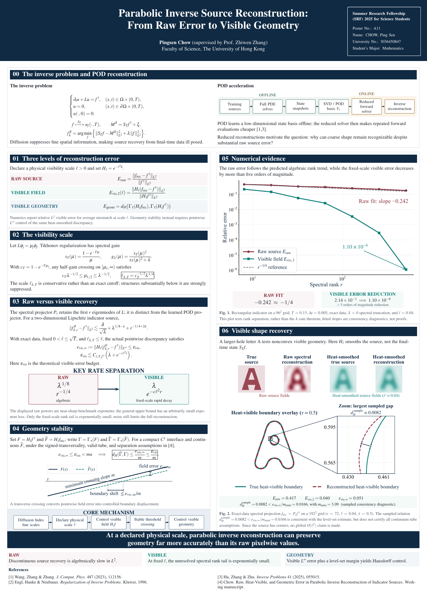
How much can we recover from temperature measurements after heat has spread? I study source reconstruction and smaller models that make repeated solves faster.
HKU Summer Research Fellowship · Faculty of Science, The University of Hong Kong · 2026
Supervisor: Prof. Zhiwen Zhang
Updated News: Selected as one of the best poster presenters and invited to present at the HKU Science Undergraduate Research Colloquium (Summer 2026).
Finding a hidden heat source
Heat spreads and blurs the evidence. Can we work backwards from the final temperature to find where it came from?
This 34-second video follows three models as they recover a hidden letter A from the same noisy measurements. Proper orthogonal decomposition (POD) learns a compact model from examples, reducing the number of values the solver needs to adjust.
Open video in a new tab · Text transcript
What to look for
The model trained on letters finishes quickly and keeps the A’s legs and opening. The model trained on circles is also fast, but distorts that shape. The full model takes longer and gives the most accurate outline in this example.
| Model | Values adjusted | Iterative solve | Shape overlap |
|---|---|---|---|
| Full model | 961 | 5.56 s | 92% |
| POD trained on letters | 14 | 48 ms | 84% |
| POD trained on circles | 13 | 56 ms | 55% |
On narrow screens, scroll the table sideways to see every column.
The takeaway: a compact model can save computation when its training examples cover the shapes we want to recover. Here, the letter-trained model is about 116 times faster in the iterative solve, with a loss in accuracy.
“Shape overlap” compares the recovered and reference regions after smoothing at the same physical scale: their shared area divided by their combined area. A is included in the letter training set, so this example shows recovery of a represented shape.
How the comparison was made
All three models use the same source, measurements, noise, mesh, time step, regularization, visibility scale, and iterative solver (steepest descent with exact line search). The video uses recorded solver iterations. It slows the opening, pauses when both POD models finish, then accelerates the remaining replay tenfold. This playback change is separate from the measured 116-fold solve-time difference.
The timings include forming the data right-hand side, solving for coefficients, and mapping the solution back to the full grid. Offline training, operator assembly, and video rendering are excluded. Cached direct solves are faster for this linear quadratic problem: 10.60 ms for the full model, 0.0423 ms for letter-trained POD, and 0.0378 ms for circle-trained POD, measured separately over 40 queries. The video’s speedup applies to iterative optimization.
This is one preselected noise realization, not evidence of performance on unseen letters. It is a finite-element/POD experiment.
Setup: a 32 × 32-cell mesh with 961 interior unknowns; final time 1; time step 1/32; 100 × 100 sensors; regularization 10−6; Gaussian noise standard deviation 10−3; visibility length 0.08/π.
Research overview
Heat spreads out over time, blurring the shape of the source that produced it. My research asks how we can work backwards from temperature measurements to recover the source’s location and shape.
I use numerical models of heat diffusion and compare full-sized solvers with reduced models built using proper orthogonal decomposition (POD). POD learns a compact representation from examples, so repeated reconstructions can adjust fewer values.
The demo follows three models through the same letter-A reconstruction. I compare the recovered values, the visible outline and the computation time to understand what each model captures.
Research materials